4. Tutorials

The following is a basic tutorial about the use of the Semi-Automatic Classification Plugin. Using a semi-automatic approach we are going to rapidly classify a Landsat 8 image and estimate land cover area, in only six phases.

Download the sample dataset, which is a subset of a Landsat 8 image acquired over Rome, Italy on June 12, 2014 (data available from the U.S. Geological Survey). The zip file can be extracted with any file archiver software (for instance the open source 7-zip).

The dataset includes the metadata file (MTL.txt) and the following Landsat 8 bands (16 bit raster) :

• Band 2 = Blue;
• Band 3 = Green;
• Band 4 = Red;
• Band 5 = Near-Infrared;
• Band 6 = Short Wavelength Infrared 1;
• Band 7 = Short Wavelength Infrared 2.

The objective of this tutorial is to classify the following land cover classes:

• Class 1 = Water (e.g. surface water);
• Class 2 = Vegetation (e.g. grassland or trees);
• Class 3 = Built-up (e.g. artificial areas, buildings and asphalt);
• Class 4 = Bare soil (e.g. soil without vegetation).

Following, the tutorial phases are illustrated along with a brief description thereof.

4.1. Pre processing: Conversion of raster bands from DN to Reflectance

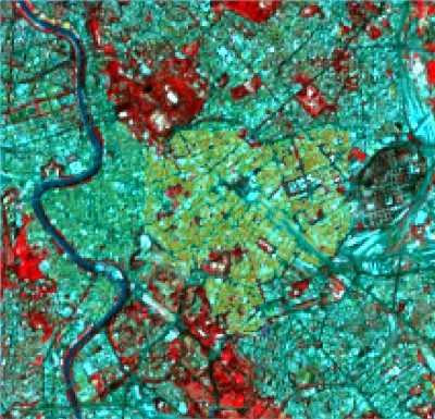
The pre processing phase is required before the actual image processing in order to improve the classification results. SCP allows for the automated conversion of Landsat DN (i.e. Digital Numbers) to the physical measure of Top Of Atmosphere reflectance (TOA, see Basic Definitions). Also, SCP implements an image-based atmospheric correction using the DOS1 method (Dark Object Subtraction 1) as described in Landsat image conversion to reflectance and DOS1 atmospheric correction. In addition, we are going to create a color composite of the image. In particular, the composite RGB = 543 (that is the equivalent of RGB = 432 for Landsat 7) is useful for the interpretation of the image because vegetation pixels appear red (healthy vegetation reflects a large part of the incident light in the near-infrared wavelength, resulting in higher reflectance values for band 5, thus higher values for the associated color red).

Steps:

• Open QGIS and start the Semi-Automatic Classification Plugin;
• Select the Вкладка Передоброблення (Pre processing) > Вкладка Landsat;

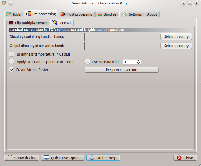
• Select the directory that contains the Landsat bands (and also the required metafile MTL.txt), and select the output directory where converted bands are saved;
• Check the option Apply DOS1 atmospheric correction, and click Perform conversion to convert Landsat bands to reflectance (leaving checked Create Virtual Raster);

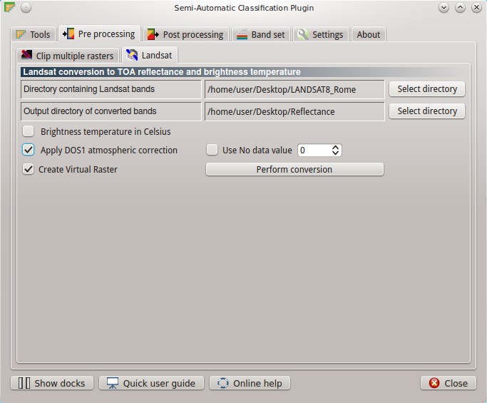
• At the end of the process, converted bands are loaded in QGIS. Also, a virtual raster named landsat.vrt is loaded (containing all the Landsat bands converted to reflectance), which is useful for the creation of color composites;
• Select the Landsat virtual raster, left click and open its properties; in Style select band 4 (i.e. Near-Infrared) for the red band, band 3 (i.e. Red) for the green band, and band 2 (i.e. Green) for the blue band.

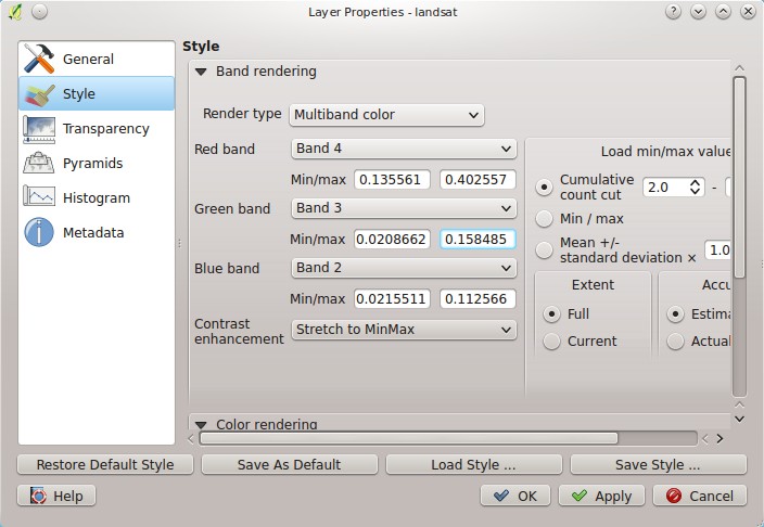
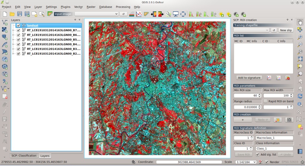
The result of the color composite is shown in the following image.

4.2. Definition of the classification inputs

We need to define the input image (i.e. the Landsat bands), the training shapefile (for the ROI collection), and the signature list file (which stores the spectral signatures calculated from ROIs or imported from other sources) in SCP.

Steps:

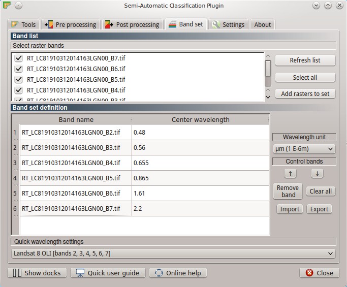
• Select the Вкладка Набір каналів (Band set) (also, a button is available in the SCP Панель інструментів); click the button Select All, then Add rasters to set (order the band names in ascending order, from top to bottom using the arrow buttons); then, select the Landsat 8 OLI from the combo box Quick wavelength settings, in order to set automatically the center wavelength of bands.

• In order to create the training shapefile, in the Панель Створення ROI (ROI Creation) click the button New shp, and select where to save the shapefile (for instance ROI.shp);
• Click the button Save in the Панель Класифікації (Classification), in order to create a signature list file (for instance SIG.xml).

In the SCP Панель інструментів, the name << band set >> is displayed in the combo box Input image. The shapefile name is displayed in the Навчальний шейп-файл (Training shapefile) combo box, and the path to the xml file is displayed in the Файл переліку сигнатур (Signature list file). Now we are ready to collect the ROIs.

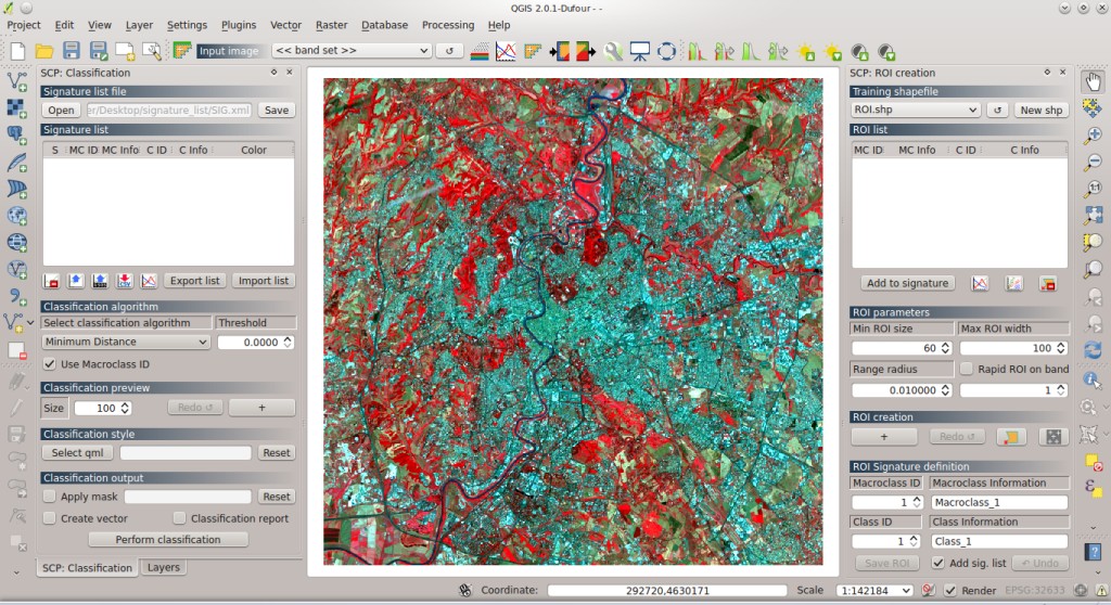
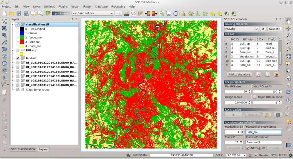
4.3. Collection of ROIs and Spectral Signatures

ROIs are polygons drawn over homogeneous areas of the image that represent land cover classes. ROIs can be drawn manually or with a region growing process (i.e. image segmentation that groups similar pixels), and they should account for the spectral variability of land cover classes. SCP calculates the spectral signatures (which are used by classification algorithms) considering the pixel values under each ROI. SCP allows for the definition of a Macroclass ID (i.e. MC ID) and a Class ID (i.e. C ID) for each ROI or spectral signature, which are the identification codes of land cover classes. A Macroclass is a group of ROIs having different Class ID, which is useful when one needs to classify materials that have different spectral signatures in the same land cover class. For instance we could classify grass (e.g. ID class = 1 and Macroclass ID = 1 ) and trees (e.g. ID class = 2 and Macroclass ID = 1 ) as a vegetation class (e.g. Macroclass ID = 1 ) as shown in Figure Macroclass example.

Macroclass example

Every ROI (or spectral signature) should have a unique C ID, while the MC ID can be shared with other ROIs. In the Панель Класифікації (Classification) it is possible to choose between MC ID and C ID classification.

Steps:

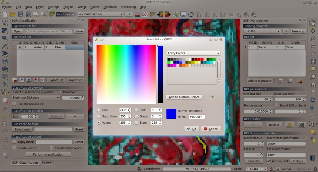
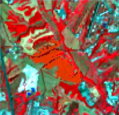
• In order to create a ROI, in the dock Панель Створення ROI (ROI Creation) click the button + beside Create a ROI and then click any pixel of the image; zoom in the map and click on a blue pixel of the Tiber river (in order to define the ROI extent, change the Параметри ROI (ROI parameters) for Min ROI size and Range radius); after a few seconds the ROI polygon will appear over the image (a semitransparent orange polygon);

  Tip: ROIs are placed inside a group named Class_temp_group; if no ROI is displayed, move the group on top of other layers in QGIS.

• Under Визначення сигнатур ROI (ROI Signature definition) type a brief description of the ROI inside the field C Info and MC Info, and assign a Macroclass ID and Class ID (these codes can renamed and changed later from the Перелік ROI (ROI list) table, thus changing also the values in the training shapefile);
• In order to save the ROI to the training shapefile click the button Save ROI; if the checkbox Add sig. list is checked, then the spectral signature is calculated and added to the Перелік сигнатур (Signature list) table; also, it is possible to add signatures later, highlighting the ROIs in the Перелік ROI (ROI list) and clicking Add to signature (if two or more highlighted ROIs have the same MC ID and C ID, a unique spectral signature is calculated considering all the pixels that are under those ROIs);

• Define the color of classes that will be used in the classification, with a double click on the Color column in the Перелік сигнатур (Signature list) (the signature list is automatically saved when you save the QGIS project, or when you click the button Save in the Панель Класифікації (Classification)).

Repeat the above steps for every land cover class, and assign to each ROI a new incremental Class ID, and the following Macroclass IDs:

• Water (e.g. surface water): MC ID = 1
• Vegetation (e.g. grassland or trees): MC ID = 2
• Built-up (e.g. artificial areas, buildings and asphalt): MC ID = 3
• Bare soil (e.g. soil without vegetation): MC ID = 4

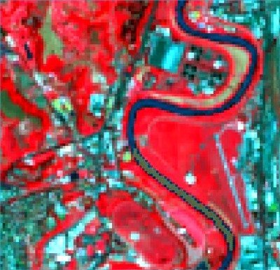
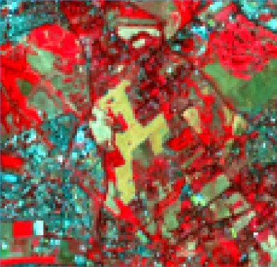
Following, a few examples of ROIs created for these land cover classes.

Bare soil

Vegetation: trees

Vegetation: grass

Built-up

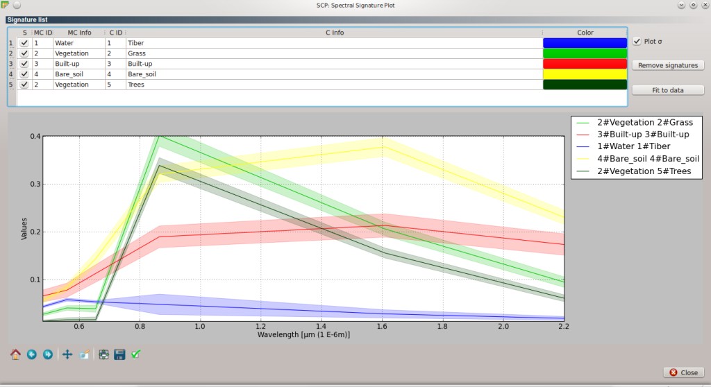
After the collection of several ROIs, it is useful to display the spectral signatures thereof, in order to assess the spectral similarity:

• In the Перелік сигнатур (Signature list) table, highlight one or more signatures, and click the button ; in the Графік спектральних сигнатур (Spectral Signature Plot), if the checkox Plot \(\sigma\) is checked, then the plot will display the standard deviation of signatures.

You can download the final training shapefile and spectral signature list, where 11 spectral signatures were collected.

4.4. Classification of the study area

SCP allows for classification previews, in order to assess very rapidly the classification results. Classifications previews are useful during the collection of ROIs, and for the selection of the more accurate spectral signatures. If the preview results are considered good (i.e. classes are correctly identified), the classification of the entire image can be performed. Otherwise, it is possible to remove one or more spectral signatures, or add new spectral signatures creating other ROIs as described in Collection of ROIs and Spectral Signatures.

Steps:

• In the Панель Класифікації (Classification), under Попередній перегляд результатів класифікації (Classification preview) set Size = 500 (i.e. the side of the classification preview in pixel unit), and select the algorithm Spectral Angle Mapping; click the button + and then click on the image; after a few seconds, the classification preview will be displayed;

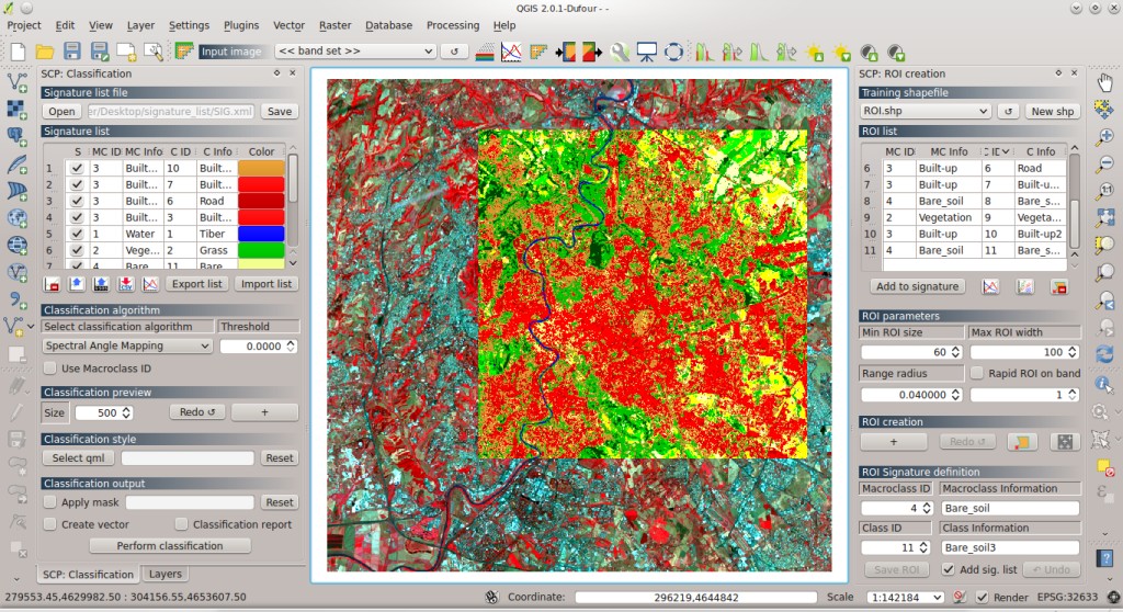
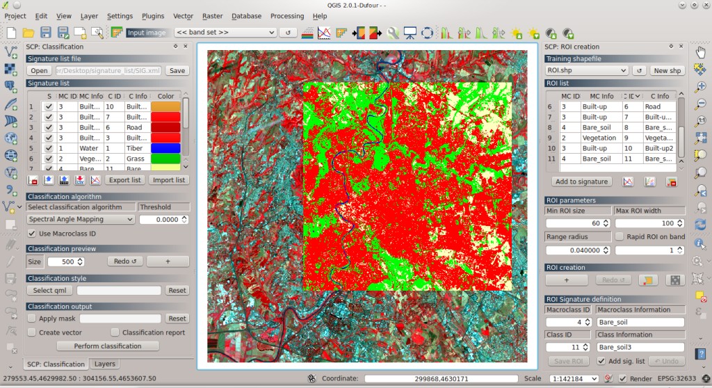
• Check Use Macroclass ID, and click the button Redo; another preview will be performed, but now using macroclasses;

• In order to perform the final classification, click the button Perform classification and select where to save the output (e.g. classification.tif).

The final land cover classification can be downloaded from here.

Tip: during the ROI/Signature collection, perform some classification previews using the Class ID, in order to assess how individual spectral signatures affect the classification; then check Use Macroclass ID, in order to calculate the final land cover classification.

4.5. Calculation of classification accuracy

The accuracy assessment of land cover classification is useful for identifying map errors. SCP allows for the calculation of accuracy comparing the classification raster to a reference shapefile. Usually, accuracy assessment requires ancillary data and field survey. In this tutorial we are are going to compare the land cover classification to the training ROIs.

Steps:

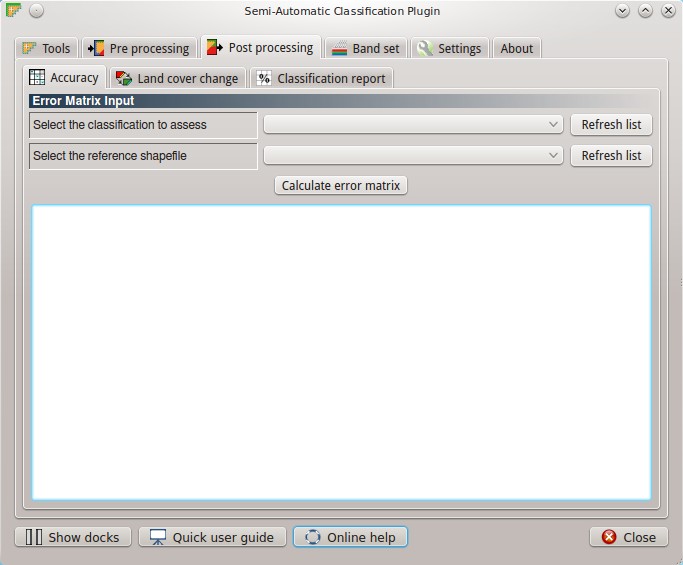
• Select the Вкладка Післяоброблення (Post processing) > Вкладка Точність (Accuracy);

• Select the classification.tif beside Select the classification to assess and select the ROI shapefile beside Select the reference shapefile;
• Click the button Calculate error matrix and select a directory where the error matrix (a .csv file separated by tab) and the error raster are saved; the error matrix will be displayed, and the error raster will be loaded in QGIS, showing the errors in the map (each value of this raster represents a class of comparison between classification and reference shapefile, which is the ErrorMatrixCode in the error matrix file).

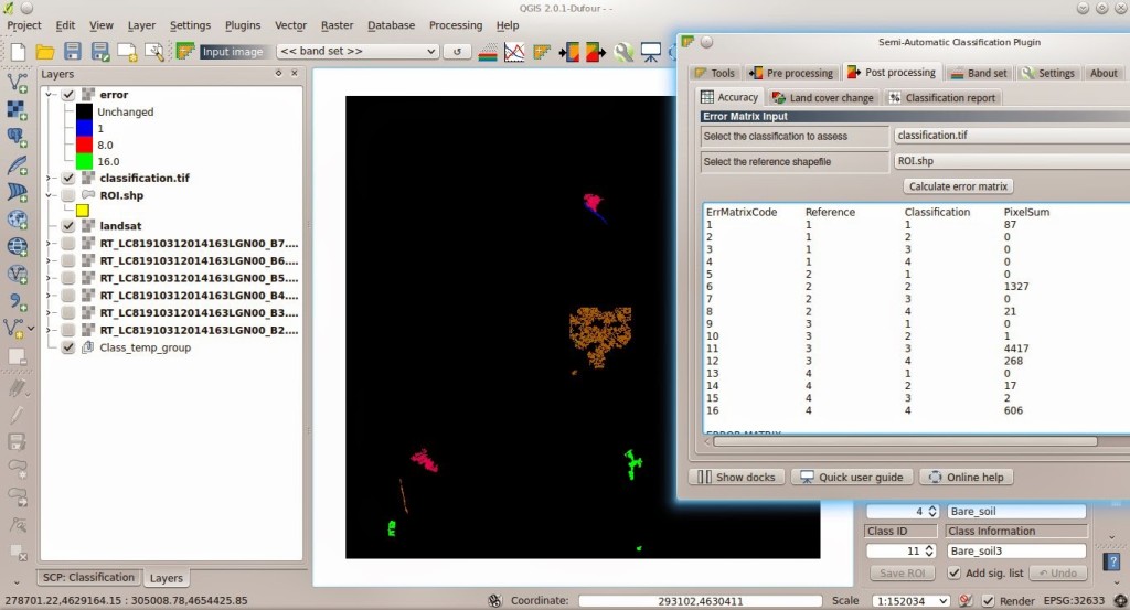
The results of the error matrix show an overall accuracy of 95%, which is very good. The following error matrix represents the number of pixels classified correctly in the major diagonal. As you can see, most of the errors are between class 3 (built-up) and 4 (bare soil).

	Reference
Classification	1	2	3	4	Total
1	87	0	0	0	87
2	0	1327	1	17	1345
3	0	0	4417	2	4419
4	0	21	268	606	895
Total	87	1348	4686	625	6746

From the error matrix file, we have also calculated the accuracy of user and producer; the results show that class 4 (bare soil) has high commission error (100 - user accuracy) and low omission error (100 - producer accuracy). In order to improve the results, we should collect more ROIs and spectral signatures for the bare soil class, paying attention to the spectral similarity with the built-up class.

• Class 1: producer accuracy [%] = 100.0; user accuracy [%] = 100.0
• Class 2: producer accuracy [%] = 98.44; user accuracy [%] = 98.66
• Class 3: producer accuracy [%] = 94.26; user accuracy [%] = 99.96
• Class 4: producer accuracy [%] = 96.96; user accuracy [%] = 67.71

4.6. Calculation of the area of classes

SCP allows for the calculation of a classification report with the percentage and the area of land cover classes.

Steps:

• Select the Вкладка Післяоброблення (Post processing) > Вкладка Звіт про результати класифікації (Classification report);

• Select classification.tif beside Select the classification and click Calculate classification report;
• After a few seconds the report will be displayed, showing the percentage and the area (area unit is calculated from the image itself).

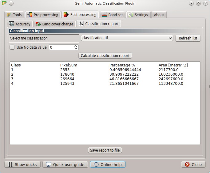
Following, the report table.

Class	PixelSum	Percentage %	Area [metre^2]
1	2353	0.41	2117700
2	178040	30.91	160236000
3	269664	46.82	242697600
4	125943	21.86	113348700

From these results, we can see that about 31% of the study area is vegetated, 47% is occupied by built-up, 22% is bare soil surface (also in agricultural areas), and 0.4% is surface water. Of course, these figures are the result of a tutorial for demonstrating the main features of the SCP for the land cover classification of a Landsat image; several ROIs for each class are required for a good classification (only 11 ROIs were collected in this tutorial), considering their spectral variability; also, field data is useful for improving the collection of ROIs and spectral signatures.

Following the video of this tutorial.

http://www.youtube.com/watch?v=Uq2S3_InQ8A

Please, visit the blog From GIS to Remote Sensing for other tutorials such as:

• Estimation of Land Surface Temperature with Landsat Thermal Infrared Band;
• Land Cover Classification of Cropland.