3. Brief Introduction to Remote Sensing
3.1. Basic Definitions
This chapter provides basic definitions about GIS and remote sensing, as a quick reference for the following tutorials.
There are several definitions of GIS (Geographic Information Systems), which is not simply a program. In general, GIS are systems that allow for the use of geographic information (data have spatial coordinates). In particular, GIS allow for the view, query, calculation and analysis of spatial data, which are mainly distinguished in raster or vector data structures. Vector is made of objects that can be points, lines or polygons, and each object can have one ore more attribute values; a raster is a grid (or image) where each cell has an attribute value (Fisher and Unwin, 2005). Several GIS applications use raster images that are derived from remote sensing.
A general definition of Remote Sensing is “the science and technology by which the characteristics of objects of interest can be identified, measured or analyzed the characteristics without direct contact” (JARS, 1993).
Usually, remote sensing is the measurement of the energy that is emanated from the Earth’s surface. If the source of the measured energy is the sun, then it is called passive remote sensing, and the result of this measurement can be a digital image (Richards and Jia, 2006). If the measured energy is not emitted by the Sun but from the sensor platform then it is defined as active remote sensing, such as radar sensors which work in the microwave range (Richards and Jia, 2006).
The electromagnetic spectrum is “the system that classifies, according to wavelength, all energy (from short cosmic to long radio) that moves, harmonically, at the constant velocity of light” (NASA, 2013). Passive sensors measure energy from the optical regions of the electromagnetic spectrum: visible, near infrared (i.e. IR), short-wave IR, and thermal IR (see Figure Electromagnetic-Spectrum).
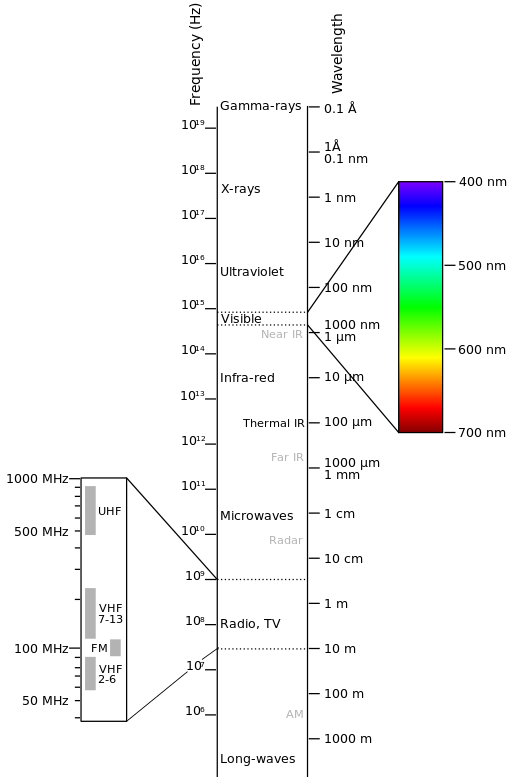
Electromagnetic-Spectrum
by Victor Blacus (SVG version of File:Electromagnetic-Spectrum.png)
[CC-BY-SA-3.0 (http://creativecommons.org/licenses/by-sa/3.0)]
via Wikimedia Commons
http://commons.wikimedia.org/wiki/File%3AElectromagnetic-Spectrum.svg
The interaction between solar energy and materials depends on the wavelength; solar energy goes from the Sun to the Earth and then to the sensor. Along this path, solar energy is (NASA, 2013):
- Transmitted - The energy passes through with a change in velocity as determined by the index of refraction for the two media in question.
- Absorbed - The energy is given up to the object through electron or molecular reactions.
- Reflected - The energy is returned unchanged with the angle of incidence equal to the angle of reflection. Reflectance is the ratio of reflected energy to that incident on a body. The wavelength reflected (not absorbed) determines the color of an object.
- Scattered - The direction of energy propagation is randomly changed. Rayleigh and Mie scatter are the two most important types of scatter in the atmosphere.
- Emitted - Actually, the energy is first absorbed, then re-emitted, usually at longer wavelengths. The object heats up.
Sensors can be on board of airplanes or on board of satellites, measuring the electromagnetic radiation at specific ranges (usually called bands). As a result, the measures are quantized and converted into a digital image, where each picture elements (i.e. pixel) has a discrete value in units of Digital Number (DN) (NASA, 2013). The resulting images have different characteristics (resolutions) depending on the sensor. There are several kinds of resolutions:
- Spatial resolution, usually measured in pixel size, “is the resolving power of an instrument needed for the discrimination of features and is based on detector size, focal length, and sensor altitude” (NASA, 2013); spatial resolution is also referred to as geometric resolution or IFOV;
- Spectral resolution, is the number and location in the electromagnetic spectrum (defined by two wavelengths) of the spectral bands (NASA, 2013) in multispectral sensors, for each band corresponds an image;
- Radiometric resolution, usually measured in bits (binary digits), is the range of available brightness values, which in the image correspond to the maximum range of DNs; for example an image with 8 bit resolution has 256 levels of brightness (Richards and Jia, 2006);
- For satellites sensors, there is also the temporal resolution, which is the time required for revisiting the same area of the Earth (NASA, 2013).
For example, Landsat is a multispectral family of satellites developed by the NASA (National Aeronautics and Space Administration of USA), very used for environmental research. The resolutions of Landsat 7 sensor are reported in the following table (from http://landsat.usgs.gov/band_designations_landsat_satellites.php); also, Landsat temporal resolution is 16 days (NASA, 2013).
| Landsat 8 Bands | Wavelength (micrometers) | Resolution (meters) |
|---|---|---|
| Band 1 - Coastal aerosol | 0.43 - 0.45 | 30 |
| Band 2 - Blue | 0.45 - 0.51 | 30 |
| Band 3 - Green | 0.53 - 0.59 | 30 |
| Band 4 - Red | 0.64 - 0.67 | 30 |
| Band 5 - Near Infrared (NIR) | 0.85 - 0.88 | 30 |
| Band 6 - SWIR 1 | 1.57 - 1.65 | 30 |
| Band 7 - SWIR 2 | 2.11 - 2.29 | 30 |
| Band 8 - Panchromatic | 0.50 - 0.68 | 15 |
| Band 9 - Cirrus | 1.36 - 1.38 | 30 |
| Band 10 - Thermal Infrared (TIRS) 1 | 10.60 - 11.19 | 100 (resampled to 30) |
| Band 11 - Thermal Infrared (TIRS) 2 | 11.50 - 12.51 | 100 (resampled to 30) |
Often, a combination is created of three individual monochrome images, in which each is assigned a given color; this is defined color composite and is useful for photo interpretation (NASA, 2013). Color composites are usually expressed as
“R G B = Br Bg Bb”
where:
- R stands for Red;
- G stands for Green;
- B stands for Blue;
- Br is the band number associated to the Red color;
- Bg is the band number associated to the Green color;
- Bb is the band number associated to the Blue color.
The following Figure Color composite of a Landsat 8 image shows a color composite “R G B = 4 3 2” of a Landsat 8 image (for Landsat 7 it is 3 2 1) and a color composite “R G B = 5 4 3” (for Landsat 7 it is 4 3 2). The composite “R G B = 5 4 3” is useful to identify vegetation, because it is clearly highlighted in red.
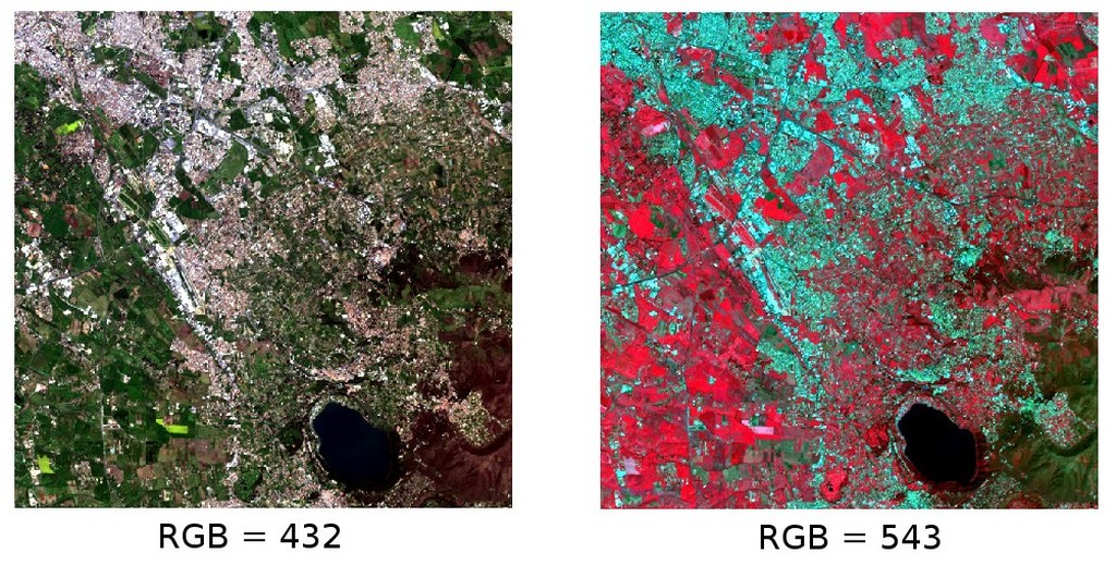
Color composite of a Landsat 8 image
Data available from the U.S. Geological SurveySensors measure the radiance, which corresponds to the brightness in a given direction toward the sensor; it useful to define also the reflectance as the ratio of reflected versus total power energy. The spectral signature is the reflectance as a function of wavelength (see Figure Spectral Reflectance Curves of Four Different Targets); each material has a unique signature, therefore it can be used for material classification (NASA, 2013).
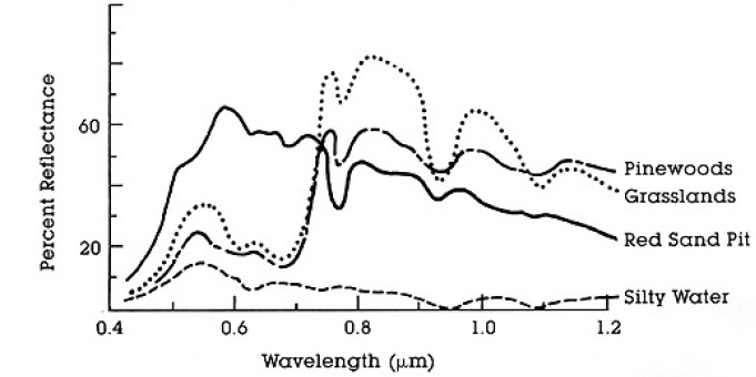
Spectral Reflectance Curves of Four Different Targets
(from NASA, 2013)A semi-automatic supervised classification is an image processing technique that allows for the identification of materials in an image, according to their spectral signatures. There are several kinds of classification algorithms, but the general purpose is to produce a thematic map of the land cover.
Land cover is the material at the ground, such as soil, vegetation, water, asphalt, etc. (Fisher and Unwin, 2005). Depending on the sensor resolutions, the number and kind of land cover classes that can be identified in the image can vary significantly.
Image processing and GIS spatial analyses require specific software such as the Semi-Automatic Classification Plugin for QGIS.
Usually, supervised classifications require the user to select one or more Regions of Interest (ROIs) for each land cover class. ROIs are polygons defined over the image that overlay pixels belonging to the same land cover class identified with an ID code (i.e. Identifier). After ROI collection, spectral characteristics of land cover classes are calculated considering the values of each pixel belonging to the ROIs that have the same class ID. Therefore, the classification algorithm classifies the whole image by calculating the spectral characteristics of each pixel, and comparing them to the defined land cover classes.
The result of the classification process is a raster (see an example of Landsat classification in Figure Landsat classification), where pixel values correspond to class IDs. Of course, there can be errors in the land cover classification (i.e. pixels assigned to a wrong land cover class), due to spectral similarity of classes, or wrong class definition during the ROI collection.
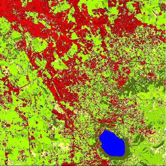
Landsat classification
Data available from the U.S. Geological SurveyAfter the classification process, it is useful to assess the accuracy of land cover classification, in order to identify and measure map errors. Usually, accuracy assessment is performed with the calculation of an error matrix, which is a table that compares map information with reference data (i.e. ground truth data) for a number of sample areas (Congalton and Green, 2009).
The following table is a scheme of error matrix, where k is the number of classes identified in the land cover classification, and n is the total number of collected sample units. The items in the major diagonal (aii) are the number of samples correctly identified, while the other items are classification error.
| Ground truth 1 | Ground truth 2 | … | Ground truth k | Total | |
|---|---|---|---|---|---|
| Class 1 | \(a_{11}\) | \(a_{12}\) | … | \(a_{1k}\) | \(a_{1+}\) |
| Class 2 | \(a_{21}\) | \(a_{22}\) | … | \(a_{2k}\) | \(a_{2+}\) |
| … | … | … | … | … | … |
| Class k | \(a_{k1}\) | \(a_{k2}\) | … | \(a_{kk}\) | \(a_{k+}\) |
| Total | \(a_{+1}\) | \(a_{+2}\) | … | \(a_{+k}\) | \(n\) |
Therefore, it is possible to calculate the overall accuracy as the ratio between the number of samples that are correctly classified (the sum of the major diagonal), and the total number of sample units n (Congalton and Green, 2009).
For further information, the following documentation is freely available: Landsat 7 Science Data User’s Handbook, Remote Sensing Note , or Wikipedia.
References
- Congalton, R. and Green, K., 2009. Assessing the Accuracy of Remotely Sensed Data: Principles and Practices. Boca Raton, FL: CRC Press.
- Fisher, P. F. and Unwin, D. J., eds. 2005. Representing GIS. Chichester, England: John Wiley & Sons.
- JARS, 1993. Remote Sensing Note. Japan Association on Remote Sensing. Available at http://www.jars1974.net/pdf/rsnote_e.html
- NASA, 2013. Landsat 7 Science Data User’s Handbook. Available at http://landsathandbook.gsfc.nasa.gov
- Richards, J. A. and Jia, X., 2006. Remote Sensing Digital Image Analysis: An Introduction. Berlin, Germany: Springer.
3.2. Landsat image conversion to reflectance and DOS1 atmospheric correction
Radiance is the “flux of energy (primarily irradiant or incident energy) per solid angle leaving a unit surface area in a given direction”, “Radiance is what is measured at the sensor and is somewhat dependent on reflectance” (NASA, 2011, p. 47).
The Spectral Radiance at the sensor’s aperture (\(L_{\lambda}\)) is measured in [watts/(meter squared * ster * \(\mu m\))] and for Landsat images it is given by (https://landsat.usgs.gov/Landsat8_Using_Product.php):
where:
- \(M_{L}\) = Band-specific multiplicative rescaling factor from Landsat metadata (RADIANCE_MULT_BAND_x, where x is the band number)
- \(A_{L}\) = Band-specific additive rescaling factor from Landsat metadata (RADIANCE_ADD_BAND_x, where x is the band number)
- \(Q_{cal}\) = Quantized and calibrated standard product pixel values (DN)
“For relatively clear Landsat scenes, a reduction in between-scene variability can be achieved through a normalization for solar irradiance by converting spectral radiance, as calculated above, to planetary reflectance or albedo. This combined surface and atmospheric reflectance of the Earth is computed with the following formula” (NASA, 2011, p. 119):
where:
- \(\rho_{p}\) = Unitless planetary reflectance, which is “the ratio of reflected versus total power energy” (NASA, 2011, p. 47)
- \(L_{\lambda}\) = Spectral radiance at the sensor’s aperture (at-satellite radiance)
- \(d\) = Earth-Sun distance in astronomical units (provided with Landsat 8 metafile, and an excel file is available from http://landsathandbook.gsfc.nasa.gov/excel_docs/d.xls)
- \(ESUN_{\lambda}\) = Mean solar exo-atmospheric irradiances
- \(\theta_{s}\) = Solar zenith angle in degrees, which is equal to \(\theta_{s}\) = 90° - \(\theta_{e}\) where \(\theta_{e}\) is the Sun elevation
It is worth pointing out that Landsat 8 images are provided with band-specific rescaling factors that allow for the direct conversion from DN to TOA reflectance. However, the effects of the atmosphere (i.e. a disturbance on the reflectance that varies with the wavelength) should be considered in order to measure the reflectance at the ground. As described by Moran et al. (1992), the land surface reflectance (\(\rho\)) is:
where:
- \(L_{p}\) is the path radiance
- \(T_{v}\) is the atmospheric transmittance in the viewing direction
- \(T_{z}\) is the atmospheric transmittance in the illumination direction
- \(E_{down}\) is the downwelling diffuse irradiance
Therefore, we need several atmospheric measurements in order to calculate \(\rho\) (physically-based corrections). Alternatively, it is possible to use image-based techniques for the calculation of these parameters, without in-situ measurements during image acquisition.
The Dark Object Subtraction (DOS) is a family of image-based atmospheric corrections. Chavez (1996) explains that “the basic assumption is that within the image some pixels are in complete shadow and their radiances received at the satellite are due to atmospheric scattering (path radiance). This assumption is combined with the fact that very few targets on the Earth’s surface are absolute black, so an assumed one-percent minimum reflectance is better than zero percent”. It is worth pointing out that the accuracy of image-based techniques is generally lower than physically-based corrections, but they are very useful when no atmospheric measurements are available as they can improve the estimation of land surface reflectance. The path radiance is given by (Sobrino, et al., 2004):
where:
- \(L_{min}\) = “radiance that corresponds to a digital count value for which the sum of all the pixels with digital counts lower or equal to this value is equal to the 0.01% of all the pixels from the image considered” (Sobrino, et al., 2004, p. 437), therefore the radiance obtained with that digital count value (\(DN_{min}\))
- \(L_{DO1\%}\) = radiance of Dark Object, assumed to have a reflectance value of 0.01
Therfore for Landsat images:
The radiance of Dark Object is given by (Sobrino, et al., 2004):
Therefore the path radiance is:
There are several DOS techniques (e.g. DOS1, DOS2, DOS3, DOS4), based on different assumption about \(T_{v}\), \(T_{z}\) , and \(E_{down}\) . The simplest technique is the DOS1, where the following assumptions are made (Moran et al., 1992):
- \(T_{v}\) = 1
- \(T_{z}\) = 1
- \(E_{down}\) = 0
Therefore the path radiance is:
And the resulting land surface reflectance is given by:
ESUN [W /(m2 * \(\mu m\))] values for Landsat sensors are provided in the following table.
| Band | Landsat 4* | Landsat 5** | Landsat 7** |
|---|---|---|---|
| 1 | 1957 | 1983 | 1997 |
| 2 | 1825 | 1769 | 1812 |
| 3 | 1557 | 1536 | 1533 |
| 4 | 1033 | 1031 | 1039 |
| 5 | 214.9 | 220 | 230.8 |
| 7 | 80.72 | 83.44 | 84.90 |
* from Chander & Markham (2003)
** from Finn, et al. (2012)
For Landsat 8, \(ESUN\) can be calculated as (from http://grass.osgeo.org/grass65/manuals/i.landsat.toar.html):
where RADIANCE_MAXIMUM and REFLECTANCE_MAXIMUM are provided by image metadata.
References
- Chander, G. & Markham, B. 2003. Revised Landsat-5 TM radiometric calibration procedures and postcalibration dynamic ranges Geoscience and Remote Sensing, IEEE Transactions on, 41, 2674 - 2677
- Chavez, P. S. 1996. Image-Based Atmospheric Corrections - Revisited and Improved Photogrammetric Engineering and Remote Sensing, [Falls Church, Va.] American Society of Photogrammetry, 62, 1025-1036
- Finn, M.P., Reed, M.D, and Yamamoto, K.H. 2012. A Straight Forward Guide for Processing Radiance and Reflectance for EO-1 ALI, Landsat 5 TM, Landsat 7 ETM+, and ASTER. Unpublished Report from USGS/Center of Excellence for Geospatial Information Science, 8 p, http://cegis.usgs.gov/soil_moisture/pdf/A%20Straight%20Forward%20guide%20for%20Processing%20Radiance%20and%20Reflectance_V_24Jul12.pdf
- Moran, M.; Jackson, R.; Slater, P. & Teillet, P. 1992. Evaluation of simplified procedures for retrieval of land surface reflectance factors from satellite sensor output Remote Sensing of Environment, 41, 169-184
- NASA (Ed.) 2011. Landsat 7 Science Data Users Handbook Landsat Project Science Office at NASA’s Goddard Space Flight Center in Greenbelt, 186 http://landsathandbook.gsfc.nasa.gov/pdfs/Landsat7_Handbook.pdf
- Sobrino, J.; Jiménez-Muñoz, J. C. & Paolini, L. 2004. Land surface temperature retrieval from LANDSAT TM 5 Remote Sensing of Environment, Elsevier, 90, 434-440
3.3. Conversion to At-Satellite Brightness Temperature
For Landsat thermal bands, the conversion of DN to At-Satellite Brightness Temperature is given by (from https://landsat.usgs.gov/Landsat8_Using_Product.php):
where:
- \(K_{1}\) = Band-specific thermal conversion constant (in watts/meter squared * ster * \(\mu m\))
- \(K_{2}\) = Band-specific thermal conversion constant (in kelvin)
and \(L_{\lambda}\) is the Spectral Radiance at the sensor’s aperture, measured in watts/(meter squared * ster * \(\mu m\)); for Landsat images it is given by (from https://landsat.usgs.gov/Landsat8_Using_Product.php)
where:
- \(M_{L}\) = Band-specific multiplicative rescaling factor from Landsat metadata (RADIANCE_MULT_BAND_x, where x is the band number)
- \(A_{L}\) = Band-specific additive rescaling factor from Landsat metadata (RADIANCE_ADD_BAND_x, where x is the band number)
- \(Q_{cal}\) = Quantized and calibrated standard product pixel values (DN)
The \(K_{1}\) and \(K_{2}\) constant for Landsat sensors are provided in the following table:
| Constant | Landsat 4* | Landsat 5* | Landsat 7** |
|---|---|---|---|
| \(K_{1}\) (watts/meter squared * ster * \(\mu m\)) | 671.62 | 607.76 | 666.09 |
| \(K_{2}\) (Kelvin) | 1284.30 | 1260.56 | 1282.71 |
* from Chander & Markham (2003)
** from NASA (2011)
For Landsat 8, the \(K_{1}\) and \(K_{2}\) values are provided in the image metafile.
References
- Chander, G. & Markham, B. 2003. Revised Landsat-5 TM radiometric calibration procedures and postcalibration dynamic ranges Geoscience and Remote Sensing, IEEE Transactions on, 41, 2674 - 2677
- NASA (Ed.) 2011. Landsat 7 Science Data Users Handbook Landsat Project Science Office at NASA’s Goddard Space Flight Center in Greenbelt, 186 http://landsathandbook.gsfc.nasa.gov/pdfs/Landsat7_Handbook.pdf